Analysis of Algorithms
Big O notation is a mathematical notation that describes the limiting behavior of a function when the argument tends towards a particular value or infinity. It is a member of a family of notations invented by Paul Bachmann, Edmund Landau, and others, collectively called Bachmann–Landau notation or asymptotic notation.
Two simple concepts separate properties of an algorithm itself from properties of a particular computer, operating system, programming language, and compiler used for its implementation. The concepts, briefly outlined earlier, are as follows:
• The input data size, or the number n of individual data items in a single data instance to be processed when solving a given problem. Obviously, how to measure the data size depends on the problem: n means the number of items to sort (in sorting applications), number of nodes (vertices) or arcs (edges) in graph algorithms, number of picture elements (pixels) in image processing, length of a character string in text processing, and so on.
• The number of elementary operations taken by a particular algorithm, or its running time. We assume it is a function f(n) of the input data size n. The function depends on the elementary operations chosen to build the algorithm.
Algorithms are analyzed under the following assumption: if the running time of an algorithm as a function of n differs only by a constant factor from the running time for another algorithm, then the two algorithms have essentially the same time complexity. Functions that measure running time, T(n), have nonnegative values
because time is nonnegative, T(n) ≥ 0. The integer argument n (data size) is also nonnegative.
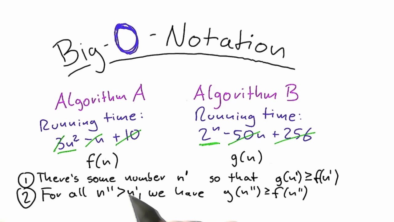
Definition 1 (Big Oh)
Let f(n) and g(n) be nonnegative-valued functions defined on nonnegative integers n. Then g(n)is O(f(n)) (read “g(n)is Big Oh of f(n)”) iff there exists a positive real constant c and a positive integer n0 such that g(n) ≤ c f(n) for all n > n0.
Note. We use the notation “iff ” as an abbreviation of “if and only if”.
In other words, if g(n)is O(f(n)) then an algorithm with running time g(n)runs for large n at most as fast, to within a constant factor, as an algorithm with running time f(n). Usually the term “asymptotically” is used in this context to describe behavior of functions for sufficiently large values of n. This term means that g(n) for large n may approach closer and closer to c · f(n). Thus, O(f(n)) specifies an asymptotic upper bound.
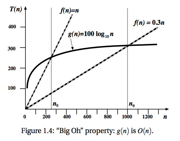
Note. Sometimes the “Big Oh” property is denoted g(n) = O(f(n)), but we should not assume that the function g(n) is equal to something called “Big Oh” of f(n). This notation really means g(n) ∈ O(f(n)), that is, g(n) is a member of the set O(f(n)) of functions which are increasing, in essence, with the same or lesser rate as n tends to infinity (n → ∞). In terms of graphs of these functions, g(n) is O(f(n)) iff there exists a constant c such that the graph of g(n) is always below or at the graph of c f(n) after a certain point, n0.
Definition 2 (Big Omega)
The function g(n) is Ω(f(n)) iff there exists a positive real constant c and a positive integer n0 such that g(n) ≥ c f(n) for all n > n0. “Big Omega” is complementary to “Big Oh” and generalizes the concept of “lower bound” (≥) in the same way as “Big Oh” generalizes the concept of “upper bound” (≤): if g(n) is O(f(n)) then f(n) is Ω(g(n)), and vice versa.
Definition 3 (Big Theta)
The function g(n) is Θ(f(n)) iff there exist two positive real constants c1 and c2 and a positive integer n0 such that c1 f(n) ≤ g(n) ≤ c2 f(n) for all n > n0.
Whenever two functions, f(n) and g(n), are actually of the same order, g(n) is Θ(f(n)), they are each “Big Oh” of the other: f(n) is O(g(n)) and g(n) is O(f(n)). In other words, f(n) is both an asymptotic upper and lower bound for g(n). The “Big Theta” property means f(n) and g(n) have asymptotically tight bounds and are in
some sense equivalent for our purposes.
In line with the above definitions, g(n) is O(f(n)) iff g(n) grows at most as fast as f(n) to within a constant factor, g(n) is Ω(f(n)) iff g(n) grows at least as fast as f(n) to within a constant factor, and g(n) is Θ(f(n)) iff g(n) and f(n) grow at the same rate to within a constant factor.
“Big Oh”, “Big Theta”, and “Big Omega” notation formally capture two crucial ideas in comparing algorithms: the exact function, g, is not very important because it can be multiplied by any arbitrary positive constant, c, and the relative behavior of two functions is compared only asymptotically, for large n, but not near the origin
where it may make no sense. Of course, if the constants involved are very large, the asymptotic behavior loses practical interest. In most cases, however, the constants remain fairly small.
In analyzing running time, “Big Oh” g(n) ∈ O(f(n)), “Big Omega” g(n) ∈ Ω(f(n)), and “Big Theta” g(n) ∈ Θ(f(n)) definitions are mostly used with g(n) equal to “exact” running time on inputs of size n and f(n) equal to a rough approximation to running time (like log n, n, n2, and so on).
To prove that some function g(n) is O(f(n)), Ω(f(n)), or Θ(f(n)) using the definitions we need to find the constants c, n0 or c1, c2, n0.
Sometimes the proof is given only by a chain of inequalities, starting with f(n). In other cases it may involve more intricate techniques, such as mathematical induction. Usually the manipulations are quite simple. To prove that g(n) is not O(f(n)), Ω(f(n)), or Θ(f(n)) we have to show the desired constants do not exist, that is, their
assumed existence leads to a contradiction.
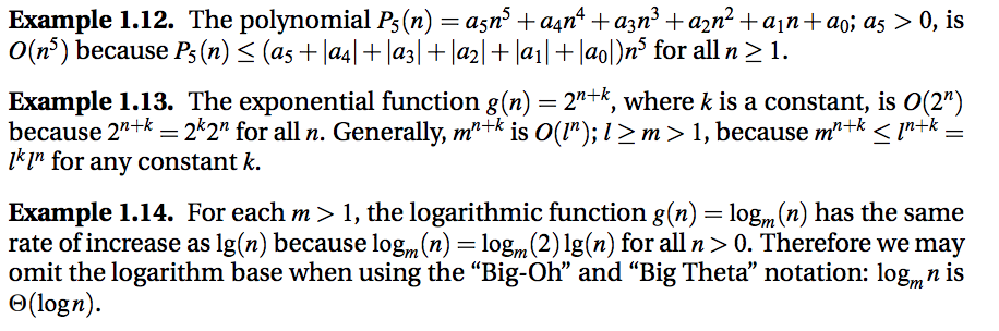
Example 1.11. To prove that linear function g(n) = an + b; a > 0, is O(n), we form the following chain of inequalities: g(n) ≤ an + |b| ≤ (a + |b|)n for all n ≥ 1. Thus, Definition 1.7 with c = a+|b| and n0 = 1 shows that an+b is O(n).
“Big Oh” hides constant factors so that both 10−10n and 1010n are O(n). It is pointless to write something like O(2n) or O(an + b) because this still means O(n). Also, only the dominant terms as n → ∞ need be shown as the argument of “Big Oh”, “Big Omega”, or “Big Theta”.
Comparing 2 different algorithms

If we wish to compare two different algorithms for the same problem, it will be very complicated to consider their performance on all possible inputs. We need a simple measure of running time. The two most common measures of an algorithm are the worst-case running time, and the average-case running time.
The worst-case running time has several advantages. If we can show, for example, that our algorithm runs in time O(n log n) no matter what input of size n we consider, we can be confident that even if we have an “unlucky” input given to our program, it will not fail to run fairly quickly. For so-called “mission-critical” applications this
is an essential requirement. In addition, an upper bound on the worst-case running time is usually fairly easy to find.
The main drawback of the worst-case running time as a measure is that it may be too pessimistic. The real running time might be much lower than an “upper bound”, the input data causing the worst case may be unlikely to be met in practice, and the constants c and n0 of the asymptotic notation are unknown and may not be small.
There are many algorithms for which it is difficult to specify the worst-case input. But even if it is known, the inputs actually encountered in practice may lead to much lower running times. We shall see later that the most widely used fast sorting algorithm, Quicksort, has worst-case quadratic running time, Θ(n2), but its running time
for “random” inputs encountered in practice is Θ(n log n).
By contrast, the average-case running time is not as easy to define. The use of the word “average” shows us that probability is involved. We need to specify a probability distribution on the inputs. Sometimes this is not too difficult. Often we can assume that every input of size n is equally likely, and this makes the mathematical
analysis easier. But sometimes an assumption of this sort may not reflect the inputs encountered in practice.
Even if it does, the average-case analysis may be a rather difficult mathematical challenge requiring intricate and detailed arguments. And of course the worst-case complexity may be very bad even if the average case complexity is good, so there may be considerable risk involved in using the algorithm. Whichever measure we adopt for a given algorithm, our goal is to show that its running time is Θ(f) for some function f and there is no algorithm with running time Θ(g) for any function g that grows more slowly than f when n → ∞. In this case our algorithm is asymptotically optimal for the given problem.
Note:
The Big-Oh notation was used as long ago as 1894 by Paul Bachmann and thenEdmund Landau for use in number theory. However the other asymptotic notations Big-Omega and Big-Theta were introduced in 1976 by Donald Knuth (at time of writing, perhaps the world’s greatest living computer scientist). Algorithms running in Θ(nlogn)time are sometimes called linearithmic, to match “logarithmic”, “linear”, “quadratic”, etc.
Source: Introduction to Algorithms, Data Structures and Formal Languages by Michael J. Dinneen, Georgy Gimel’farb, Mark C. Wilson